What matters in this issue
Start with OAT and RIFT. OAT turns successful executions into a training signal for failure localization; RIFT asks whether KV entries selected at the start remain useful during long generation. Both make changing execution state measurable. Their metrics, error-step identification and draft acceptance length, should be kept distinct from task success and serving speed.
SnakeCharmer moves down to GPU hardware, coordinating whether to issue a predicted prefetch, when to issue it, and where to retain its data. The evidence differs across the three papers: OAT includes cross-dataset diagnosis, RIFT primarily studies active-cache budgets versus drafting quality, and SnakeCharmer uses hardware simulation. Those conditions determine how far each conclusion travels.
01 · OAT: learning error-step deviations from successful trajectories
Tracing Agentic Failure from the Flow of Success
Samuel Yeh, Yiwen Zhu, Shaleen Deep, Sharon Li · First published 2026-07-14; v2 2026-10-10 · NeurIPS 2026
Learning a reference when failure labels are expensive
A wrong final answer does not identify the step that caused it. Incorrect assumptions, tool misuse, and attempted recovery can interact throughout a trajectory. Prompting an LLM to judge each step is expensive, while supervised attribution requires costly annotations. OAT uses one-class learning: train on successful executions, then flag steps that depart from their learned dynamics. The resulting candidate set can narrow an investigation.
The implementation mean-pools final-layer token representations from Qwen3.5-27B and projects them to 64 dimensions with PCA. It connects the query and step representations into a continuous path and trains a Neural CDE to reconstruct successful trajectories. A control path continually supplies observations, rather than letting the initial query determine the entire trajectory. A gate suppresses atypical control signals that could destabilize the model under distribution shift.
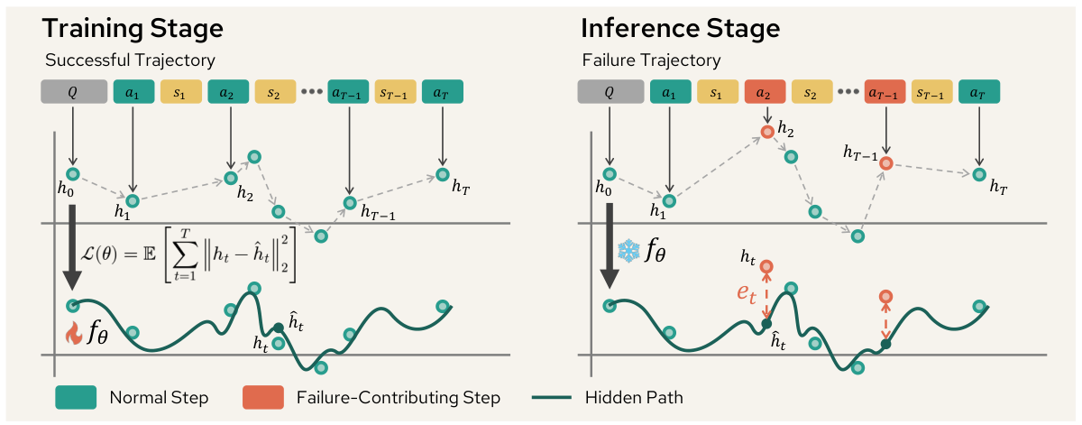
Left: learn continuous dynamics from successful traces. Right: deviations between observed steps and reconstruction identify candidate errors.
At inference, squared reconstruction distance becomes the step-level anomaly score. The authors compare selecting the top three steps with a threshold calibrated on held-out successful trajectories. Top-k has higher recall; calibration better adapts the candidate count. Its distributional assumptions also mean that false-positive control cannot simply be promised after moving to a new task distribution.
Useful localization, with limits on causal interpretation
MCP-Atlas contains 103 successful and 88 failed trajectories. Successful data are split 80%/20% for training and validation or calibration. Across five seeds, thresholded OAT reaches F1 0.435±0.013, versus 0.212 for GPT-4o and 0.181 for GPT-5. OC-SVM and Isolation Forest both reach 0.411. The improvement over prompting is substantial; the increment over classical anomaly detection is considerably smaller.
On 184 failed Who&When trajectories, Top-k OAT reaches F1 0.225 versus GPT-5’s 0.152. These trajectories were generated by GPT-4o, represented using the Qwen proxy, and aligned with unlabeled CORAL. Label semantics differ too: MCP-Atlas permits multiple contributing steps, whereas Who&When marks the earliest decisive error. This supports transfer potential without establishing one universal definition of failure attribution.
The speed claim needs its cost boundary. OAT’s reported 7/16 ms excludes hidden-state extraction. Including extraction takes approximately one second per trajectory on two H200 GPUs, giving roughly 4–35× acceleration over prompting baselines. The headline 200–5000× applies after representations are available. Nor does deviation prove that repairing a flagged step would rescue the task: the paper’s contribution-step definition does not require that counterfactual.
Read the method and cost footnote first. OAT makes inexpensive step screening an attractive diagnostic front end, particularly where hidden states are accessible. Closed-model access, task changes, and subsequent causal verification still need additional design.
02 · RIFT: keeping draft caches relevant during long generation
RIFT: KV Cache Compression for Draft Models with Complementary Compressibility Training
Dor Tsur et al. · NVIDIA · First published 2026-10-22
Importance at prefill can become stale
Speculative decoding uses a small model to propose tokens that a target verifies. Compressing the draft cache reduces its active-state footprint, but a selection made once during prefill can lose relevance as reasoning grows. The paper calls this decode staleness. In hybrid-attention models, a simple recent-token window can outperform SnapKV’s predominantly prefill-based selection.
RIFT offers three complexity levels. RIFT-stat divides capacity between important history and recent tokens, usually equally in evaluation. RIFT-dyn periodically rescores full KV history using recent queries. RIFT-ada uses acceptance length, draft entropy, and query drift to trigger refreshes, bounded by minimum and maximum intervals. The decision is which state remains worth keeping active.
Training supplies a complementary mechanism. A frozen dense draft pass scores positions and constructs a sparse attention mask combining recent tokens with important history. A trainable draft pass uses that mask with teacher labels and logits for cross-entropy and KL distillation. Limited-context conditions therefore enter training before compressed inference.
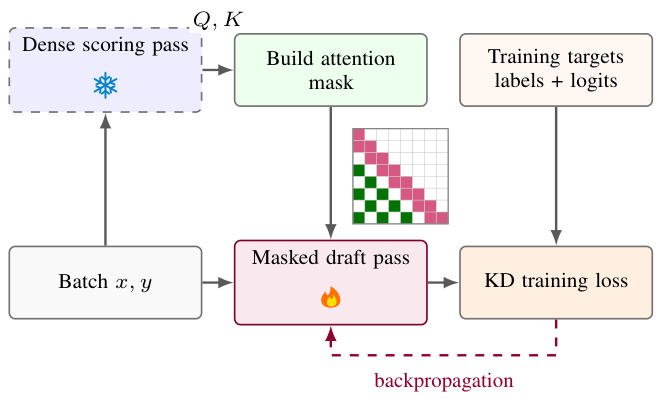
A frozen scoring pass creates a recency-and-importance mask; the trainable draft learns teacher outputs with that restricted attention.
How much acceptance length survives
On the low-entropy SPEED-Bench setting with 32K input, up to 4K output, an 8K active-cache budget, draft length 11, and temperature 0, Qwen3.5-4B drafts for Qwen3.5-122B. Average acceptance lengths are 4.07 for SnapKV, 5.23 for sliding-window attention, 5.62 for RIFT-stat, 6.12 for RIFT-dyn, and 6.19 for RIFT-ada. This metric includes the additional target-generated token; it is not final-answer accuracy.
With compression-aware training, the authors report retaining over 98% of full-cache acceptance length at 32K input, 4K output, and an 8K budget. A separate temperature-1 comparison gives approximately 51.1% fewer refreshes at comparable acceptance length, or 0.122 higher acceptance length at matched refresh count. Cache policy and draft training can reinforce each other, but these gains do not translate directly into equivalent serving acceleration.
The essential memory condition is that refresh still assumes access to full draft KV history in HBM or offloaded memory. An 8K budget describes the active working set, not total system storage. Rescoring, transfer, target verification, and drafting all contribute to latency. Some refresh-overhead analysis is projected; naive GPU measurements report overhead up to approximately 6% of draft decode latency.
Prioritize the staleness analysis and limitations. The work is most relevant to memory-constrained external drafting or self-speculation. Tail-augmented approaches such as MTP, EAGLE, and DFlash are outside the main scope and often have stronger end-to-end benefits on current GPU deployments. RIFT’s heterogeneous-serving motivation still needs complete system measurements.
03 · SnakeCharmer: turning predicted addresses into useful prefetches
SnakeCharmer: Orchestrating Utility, Timeliness, and Placement in GPU Prefetching
Yuhan Tang et al. · First published 2026-10-22 · MICRO 2026
Correct address prediction can still arrive too early, too late, or evict useful data. SnakeCharmer adds a coordinated backend: zero-value confidence filters low-value candidates, timing feedback adjusts prefetch distance, and a remapping table buffers returned data in idle registers to reduce L1 contention. That buffering can be disabled when idle capacity is unavailable.
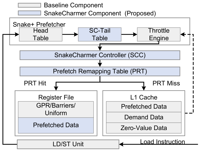
The predictor proposes candidates, the controller gates issuance, and the remapping table directs data to idle registers or L1.
Using AccelSim and AccelWattch to model A100, the authors report average IPC and performance-per-watt gains of 12.8% and 20.8% over Snake across 14 selected applications. With APOGEE, gains are 1.7% and 3.2%. Applications require ideal prediction accuracy above 50% and coverage above 30%, so the study measures realization of already available prediction opportunities. These are simulated kernel-execution results, not directly available gains on existing GPUs or LLM services.