Meta Team: Daohang Shi, Oleksandr Stashuk, Rupert Wu, Liangbei Xu, Rich Zhu
Original: Modernizing Table Batched Embeddings with FBTriton · Code
Why redesign a sparse operator?
Recommendation-model embedding tables map discrete IDs to vectors. A request can access many tables and multiple IDs within each. Table Batched Embedding (TBE) combines lookups and pooling across tables, reducing the overhead of launching a kernel for each table. The difficulty is uneven access: some rows are used once, while popular rows may be referenced thousands of times. Identically sized matrices can have very different execution bottlenecks.
FBTriton’s value lies in reorganizing the units of work, rather than translating CUDA into Python line by line. Forward execution must read and accumulate sparse rows; backward execution must gather every gradient for a row and update it exactly once. This is an engineering optimization for recommendation-system TBE, not evidence of a general speedup for ordinary LLMs.
Forward: keep a narrowly specialized path beside the general one
The generic forward path has each program loop over tables, gather indexed vectors, and pool them. FP16/BF16 weights accumulate in FP32, while FP32 weights accumulate in FP64 to reduce accumulation error at large dimensions. Configurable int32 indices are available when the linearized range fits below 2^31, reducing index and sorting costs; int64 remains the default.
Small tables can first count the occurrences of each row, then compute counts times table, converting irregular reads into tensor-core work. Eligibility is narrow: one feature with E≤64, 64≤D≤128, pooling length L≥64, FP16 weights, FP32 output, no per-sample weights, and no variable batching (VBE). A program handles 16 bags, counting the first 256 indices and using a scalar path for the remainder. Other shapes use the generic kernel.
Bounds checking remains necessary. Fused checks apply only to eligible configurations; offset validation and repair still use a separate small kernel, and the option defaults off. This gives the optimization a defined entry point and fallback instead of imposing one aggressive assumption on every input.
Backward: invert “which rows did this sample use?”
Several bags can reference the same embedding row. Backward execution must sum their output gradients before applying one optimizer update. Input transposition, sorting, and run-length encoding reorganize indices into runs: each run identifies a unique table/row pair and the samples that touched it. Segment length, SL, determines the work and can range from one to millions.
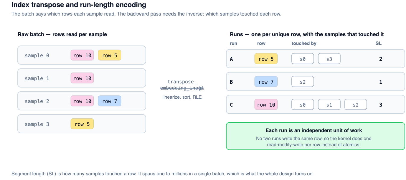
Reading the diagram: samples list their accessed rows on the left; the right groups samples by row. Row 10 has three contributing samples and becomes one independent update task of length three.
For SL<256, one program gathers, accumulates in registers, and updates the row. Exclusive ownership permits a plain store. For SL≥256, the run is split into chunks of 256 lookups. The default path stores partial sums and uses a second kernel for the update. Popular rows no longer strand the GPU behind a single long task, while short runs avoid paying for cooperation too early.
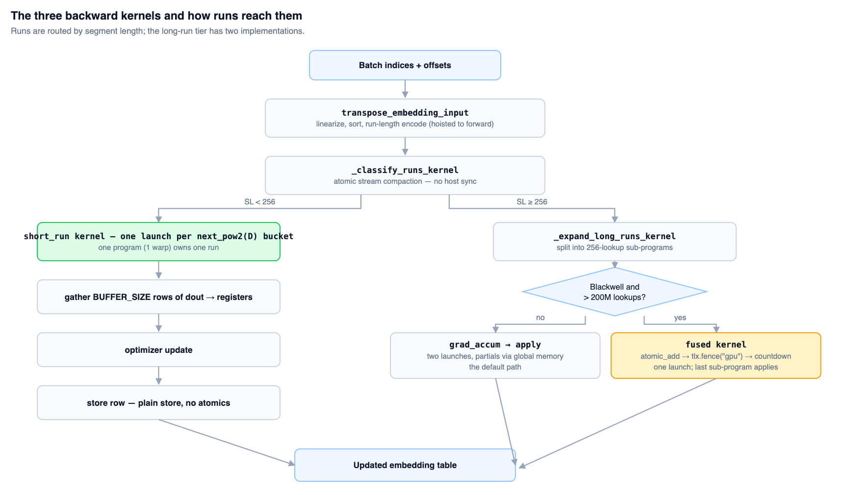
Reading the diagram: short runs take the exclusive-update path on the left; long runs split on the right. Two launches are the default, with a fused path under the illustrated Blackwell and greater-than-200-million-lookups condition. Moving preprocessing into forward is optional.
Correctness of the fused path depends on ordering: each chunk writes its partial gradient, executes a device-scope fence, and then decrements the remaining count. Only the final completing chunk may update the weights. If the count reaches zero before data becomes visible, execution may silently produce incorrect values. The article also discusses CLC work acquisition and TMA reductions, but these are hardware-specific capabilities; a Blackwell path should not be equated with the implementation on other devices.
Fewer reads and synchronizations can beat more parallel work
Buffering more rows keeps more pointers and registers live, potentially reducing occupancy. On the B200 unweighted short-run path, the authors reduce gather width from eight to two: registers fall from 184 to 64, and occupancy rises from 12.5% to 49.9%. Bucketing by next_pow2(D) separately prevents narrow tables from wasting lanes sized for the widest dimension. These address different sources of waste.
The number of long runs is only known at runtime. Reading that count back to the CPU would synchronize execution, so the implementation preallocates workspace, compacts task lists on the GPU, and has subsequent kernels consume device-resident counts. Dynamic-shape optimization must include the metadata path, not just numerical kernels.
Preprocessing can also move into forward. In one large B200 configuration, forward latency rises from 22.844 to 33.252 ms, backward falls from 56.693 to 32.931 ms, and their sum drops from 79.537 to 66.183 ms, a 16.8% reduction. This trades slower forward for a better combined result. The core-module option defaults off and is not exposed by the current TorchRec wrapper. Saving a histogram for backward reuse likewise does not mean forward and backward have fused into one launch.
Fusion boundaries are also engineering interfaces
The requirement to update once matters especially for weighted inputs: scale each gradient contribution before grouping it by row. Treating the optimizer as a backward epilogue reduces extra reads and writes; it does not authorize changing update semantics. The small-table histogram-reuse path also uses compensated FP16 high/low computation into FP32. It should not be described as merely reducing accumulation precision to gain speed.
The article presents broader sparse-kernel fusion as further opportunity. An adoption evaluation should measure input validation, transpose/sort, workspace, and optimizer execution together. Timing only the backward core can hide added forward cost, and a large speedup on one shape can conceal a tail below baseline. These are evaluation recommendations inferred from the implementation mechanisms, not additional benchmarks performed for this note.
Read results by hardware, path, and metric
The official results cover 307 shard configurations, comprising 283 distinct shapes, on GB200 with FP16 weights and exact row-wise Adagrad. The backward plot reports achieved bandwidth ratios, not full-training throughput:
| Backward configuration | Shards | Median Triton/CUDA bandwidth ratio | Share at or above CUDA |
|---|---|---|---|
| No per-sample weights | 256 | 1.13 | 94% |
| Per-sample weights | 51 | 1.22 | 69% |
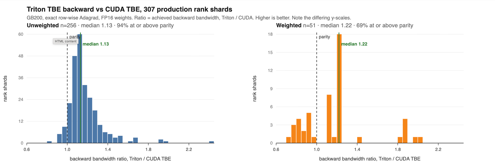
Reading the diagram: the dashed line at one marks parity. The weighted panel has a higher median but more configurations below one. Vertical scales differ; median gains and the share of configurations benefiting must both be considered.
The forward figure is separately labeled B200: Model 1 and Model 2 each have 31 measurements, with median latency speedups of 1.28 and 1.18. The prose also summarizes a 1.28× forward median; that does not justify merging both plots or all 307 configurations into one statistical population. A major backward advantage comes from CUDA switching to cooperation at SL=32 while Triton waits until 256. Shorter runs avoid synchronization that would not yet pay for itself.
Limits remain clear. The 11 of 307 shards whose work lies entirely in SL<4 runs still lose to CUDA, each taking roughly less than one millisecond. Shapes above SL=256 are approximately at parity. This is an operator-engineering account worth reading. Before migration, inspect actual run lengths, dimensions, and weighted-access distributions, then verify optimizer semantics, backend support, and combined forward/backward latency. A more editable implementation expands tuning opportunities, but easier maintenance and faster execution on every workload are separate conclusions.