vLLM Team, Inferact, Red Hat, NVIDIA · Official technical preview · 2026-10-09
Original: vLLM Support for NVIDIA Vera Rubin NVL72: 7.8x Throughput over GB200 NVL72
Read the serving curve before the hardware multipliers
The interesting development in vLLM’s Vera Rubin NVL72 support goes beyond higher throughput on a new GPU: software is beginning to place computation according to memory locality inside the GPU. The official preview discusses compatibility, specialized kernels, and locality domains. Compatibility gets models running; the other two determine how much additional compute and bandwidth becomes useful serving capacity.
The headline 7.84× comes from MiniMax M3 on AgentX, comparing per-GPU throughput against GB200 NVL72 at matched interactivity. Under a 150 TPS constraint, the same article reports 5.18×. These numbers describe different points on the performance curve and do not conflict. For interactive agents, throughput needs to be read alongside the speed at which users receive subsequent tokens.
More hardware resources do not remove every bottleneck proportionally
Relative to GB200 NVL72, the article reports approximately 5× NVFP4 FLOPS, 2.4× HBM bandwidth, and 1.7× bidirectional NVLink bandwidth, plus 2× FP32 and 4× BF16/FP16 exponential throughput. Exponentials matter for softmax, illustrating why operations beyond matrix multiplication must also keep pace.
These are not acceleration factors to multiply together. One stage may be compute-bound, another limited by weight reads, and communication may introduce further waiting. An engineering implication is to identify the constraints on prefill, decode, and communication before deciding which hardware improvement matters to a workload. Peak low-precision arithmetic alone overlooks batch size and access patterns.
Locality domains: putting operators near their weights
The article’s most concrete mechanism is CUDA 13.4 locality domains. Access costs between SMs and HBM regions inside a GPU are nonuniform. Green Contexts and CUDA streams can partition computation and keep each group of SMs reading its locally placed weight shard, reducing cross-domain accesses.
For MoE decode with few tokens, fetching expert weights from HBM dominates the forward pass. The implementation uses split-N for both FC1 and FC2: it partitions weights by columns, places the halves in two domains, and makes each domain’s kernel read its own half. Input and output activations remain accessible across both domains because their size is relatively small in this low-token regime.
The key is arranging computation and data together. Partitioning SMs while both groups remotely read all the weights might not realize the local-bandwidth advantage. Extending the small-activation assumption to large-batch prefill could also change the outcome. These are implications of the mechanism; the article does not establish equal gains for every matrix multiplication.
Domain creation also affects the available SM count. Default equal partitioning uses 200 of 212 SMs, while backfill mode uses all 212. The article compares both modes and reports approximately 1.2× average speedup for small-token forwards. Similar gains despite leaving some SMs unused support the explanation that weight loading dominates.
However, this experiment times FC1 plus FC2 per rank using MiniMax M3 shapes, balanced routing, and no communication time, across TP2, TP4, EP2, and EP4. It establishes an improvement to that MoE computation segment. It does not independently explain the full 7.84× AgentX gain or establish end-to-end results under skewed expert routing.
How layer-level gains reach user waiting time
A simple engineering estimate illustrates the boundary. Suppose the accelerated MoE layer accounts for half the original request time and everything else remains unchanged. A 1.2× layer speedup leaves total time at approximately 0.5 + 0.5 / 1.2, or 0.917 of the original: only about a 1.09× overall speedup. This is a hypothetical calculation, not a reported measurement, and excludes nonlinear changes in queueing and concurrency.
Near saturation, a small change in execution time can substantially change queues. Layer-level gains therefore neither multiply mechanically nor necessarily propagate linearly. Time to first token, subsequent output speed, and aggregate throughput need separate observation. The chart’s P90 interactivity measures output interactivity, not P90 total request latency. Treating it as complete response time would omit long-input processing and request queueing.
Precision also conditions comparisons. NVFP4 compute, FP8 KV caches, and specific checkpoints describe different configuration requirements. Higher throughput alone does not establish that precision changes preserve task quality. Deployments that must retain existing answer quality should evaluate performance and task quality separately. The throughput results in this article do not establish quality equivalence across precisions.
Running successfully and being fully optimized are different stages
Rubin introduces the sm107 compilation target while also running kernels built for the Blackwell family target sm100f. Existing GEMM, attention, and MoE paths can therefore work before hardware-specific optimization is complete. The article identifies vllm/vllm-openai:cu134-nightly, built with CUDA 13.4 and PyTorch 2.15, as its daily container, with model coverage including DeepSeek, Kimi, GLM, and MiniMax.
Rubin optimizations arrive through components including FlashInfer 0.7.0 and cover low-precision GEMM, NVFP4 MoE, FP8 attention, and MSA prefill. The appendix shows configuration dependencies: weight formats select different linear backends, FP8 attention requires an appropriate KV-cache dtype, and expert-parallel kernels depend on the deployment layout. Loading a model and actually selecting a particular fast kernel are separate states to verify.
An operational implication is that daily image tags change over time. Comparisons need a fixed image and model configuration, with precision and parallelism recorded. The article documents paths that were working at publication; it does not make every future nightly identical to the environment behind its figures.
How to read the throughput chart
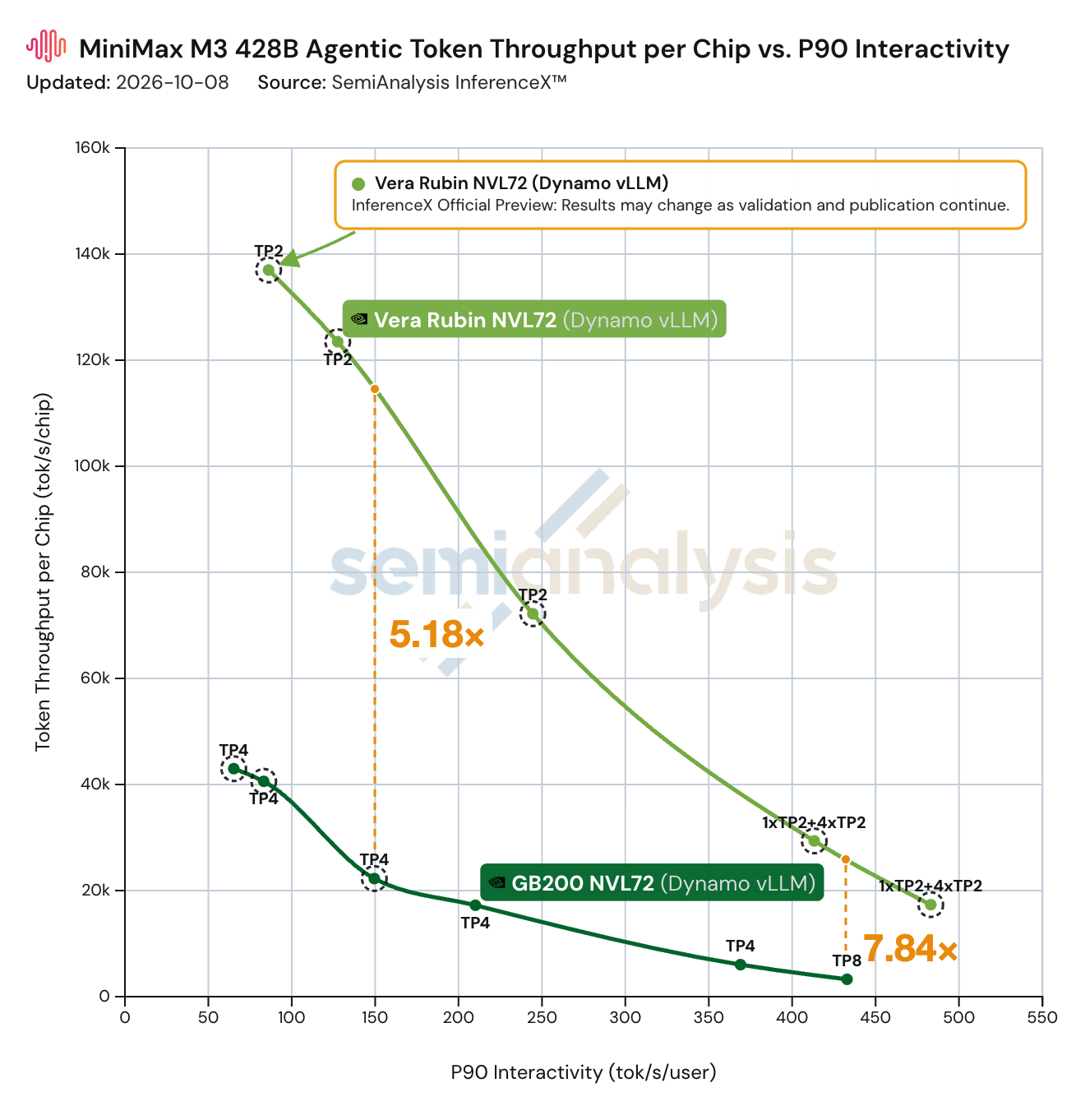
Reading the chart: the horizontal axis is P90 per-user interactivity and the vertical axis is token throughput per chip. Compare the curves at the same horizontal coordinate: 5.18× is marked at 150 TPS, and 7.84× at higher interactivity. The original parallelism labels and official-preview annotation are retained.
The curves show a trade-off between throughput and interactivity, so comparing their separate peak-throughput points would lose the service constraint. Rubin and GB200 do not use identical parallelism configurations everywhere in the chart. The result represents the combined serving capability of a platform and its software configuration; it cannot attribute all improvement to one kernel or locality domains.
A separate result comes from MLPerf Inference v6.1. With Qwen3-VL-235B-A22B as the VLM workload, vLLM as the backend, and Dynamo as the frontend router, Rubin delivers up to 3.7× the throughput of GB300 NVL72 across offline, server, and interactive scenarios. The model, benchmark protocol, and comparison hardware differ from AgentX. These multipliers should not be collapsed into a universal improvement figure.
What to follow next
The preview shows three levels of progress: compatible kernels establish usability, specialized kernels exploit new hardware capabilities, and co-placement of data and computation reduces internal access costs. For agent services, the useful question is how much more work can be served at a given interactivity target, and whether that capacity persists across different models, contexts, and routing distributions.
The article still lists full locality-domain enablement, additional MoE and attention kernels, and more inter-operator overlap as future work. Those plans should not be treated as delivered capabilities. The most useful follow-up comparisons would include complete communication costs, unbalanced expert loads, different precision configurations, and sustained throughput under fixed latency targets. The current results warrant attention, but do not supply directly convertible cost-per-unit or energy conclusions.